


Jonas Mason, Senior Consultant
Part 1 and Part 2 of this Troubleshooting Oracle Performance blog series focused on narrowing the scope and identifying problematic sessions when confronted with a general performance complaint. A troubleshooting paradigm was established to facilitate a dialogue between DBA, developer and end user. The primary objective of the dialogue is to identify problematic SQL statements and tune them. In some cases, system right sizing efforts may be appropriate and the DBA can make recommendations on whether more CPU, memory, and/or Disk I/O is required based on analysis of expensive SQL.
This final blog in the series will focus on reading explain plans and tuning SQL rather than allocating more resources to a server in order to handle inefficient SQL. It will touch on Query Diagramming, as made known by Dan Tow in his book SQL Tuning, which can be a useful non-SQL method to approach tables statistics and join costs.
Explain Plans
The Oracle Optimizer generates explain plans when a SQL statement is parsed, in order to create an access path to the underlying tables required to satisfy query results. Ideally, execution plans are simple and robust, scaling well as record counts increase over time. Robust execution plans often incorporate nested loop joins of tables, in the correct order, utilizing indexes.
Significant explain plan costs are often associated with selects that satisfy reporting and batch processes. When batch processes involve significant updates, inserts or deletes, the higher costs associated with these executions can create deadlock or hot block scenarios. I am always more concerned when I see long running DML versus long running selects for this reason. Reports that rely on significant DML activity to complete are also suspect, as they usually don’t scale well in otherwise efficient OLTP instances.
Reading an Explain Plan
SQL Developer and TOAD are among a number of tools that provide a more visual explain plan representation. Below in Figure 1, is the original explain plan for an expensive SQL statement identified in the “SQL ordered by Gets” statspack section of last week’s post. The indented lines on the right are executed first, with execution order generally scrolling left and up.
Figure 1 – Significant Cost in Explain Plan
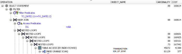
The column, Cost, in Figure 1, is important to note because this is what the optimizer is estimating as the expense to execute this line item. The top line for Cost is the total cost for the statement. The values in the cardinality column are also also valuable, as they indicate how many records are being returned for this portion of the explain plan.
As we see in this example, a higher cost can be associated with joins that result in the cardinality being reduced significantly. Why would these joins be so expensive, yet have a low cardinality value? A significant amount of work was required to evaluate the records in the join, in order to extract the smaller record set.
We know, based on a review of this statement, that the cost is primarily the result of the table access (by index row id) on the table TRANSACTION (cost 41388-377=41011, cardinality 45072), and the nested loops joining the results of TRANSACTION table with other tables being joined to below, which were not included in Figure 1. The cost of the join is 167,942-41,388 = 126,554, though its cardinality is 73. This portion of the explain plan is worth addressing primarily based on the significant portion of the total cost it represents.
Focusing on lower cost items, if they are a fraction of a percentage of the total cost of the statement, is often a waste of time. That being said, if the cardinality is higher despite a lower cost line item, and this higher cardinality contributes significantly to the expense of joins to other tables further up the explain plan, some additional attention would be warranted. This issue of cardinality could be raised with the developer or end user. The question to the end user would be what percentage of all records in the table need to be reviewed to answer the question posed? If the percentage of records in a table can be reduced, what column related criteria could be used to achieve this? Even in the far more complex case of multi table joins these questions can be directed at one table at a time.
Figure 2 – Insignificant Cost in Explain Plan
![]()
We have the option of tuning the Full Table Access to ACCOUNTS in another portion of this query’s explain plan. In Figure 2, this access path to ACCOUNT does not have a high cost (12), or result in a high cardinality value (1384). Attempting to tune access to the ACCOUNT table by adding an index, or qualifying ACCOUNTS access in the where clause, would be a waste of time. Some assume that full table scans are bad, but they aren’t necessarily. If the goal of a query is to evaluate all records in a table, the lower cost associated with a single access path to the table makes sense. So in this case, where the full table scan on the ACCOUNTS table consumes a small fraction of the total explain plan cost and cardinality is low, we can divert our attention elsewhere.
Now that we have identified the substantial sources of cost for this SQL statement, the next section addresses possible tuning options. The goal of these tuning options is to manipulate the explain plan for improved performance that results in a cost reduction.
Explain Plan Optimization
Based on the analysis above, we understand there are two problematic portions of this statement that include: 1) table access to TRANSACTION; and 2) the join between TRANSACTION and INTERFACE_LOG. The number of columns selected in a query is often not a significant contributing cost factor compared to the inefficient joins of multiple tables required to populate those columns. Extracting 10 columns of results from one table is often less expensive than extracting 10 columns of results from two or more poorly joined tables of similar size. Explain plan analysis often bears this out.
Expensive statements often are not selective enough in the Where clause which would reduce cardinality. As a result of higher cardinality, joins between tables become more expensive in the form of increased buffer gets per execution and logical block reads. More CPU and Disk I/O are consumed as a result.
Some techniques for improving explain plans, per SQL Tuning by Dan Tow, include:
- Enabling use of the index you want
- Preventing use of the wrong indexes
- Enabling the join order you want
- Preventing join orders you do not want
- Choosing the order to execute outer queries and sub queries
- Providing the cost-based optimizer with good data
Fooling the cost-based optimizer with bad data
Evaluating Index Choices
New indexes can be helpful when optimizing a select statement, but should be undertaken after or in conjunction with SQL statement structure analysis. The methods for evaluating indexes in this section inform considerations on SQL structure changes. If the cost of the access path to a table and a reduction in cardinality can be achieved , the execution time can often be decreased.
The most important portion of the query we are evaluating in this example is:
FROM interface_log eil,
transaction et,
group_xref egx,
dba.TRANSACTION cct,
group eg,
assoc_accounts aa
WHERE eil.CONTROL_NUMBER = et.CONTROL_NUMBER
AND et.TRANSACTION_NUMBER = egx.TRANSACTION_NUMBER
AND eil.CONTROL_NUMBER = cct.REFERENCE_NUMBER
AND egx.GROUP_ID = eg.GROUP_ID
AND eg.DESTINATION_ASSOC_ACCOUNT_ID = aa.ASSOC_ACCOUNTS_ID
AND eil.SERVCE_NAME IN ('ACHOOTP',
'CCOneTimePurchase',
'CCSettlement',
'PCCardSettlement',
'CCCRecurringPurchase')
AND cct.created_dt BETWEEN :1 AND :2
AND eil.assoc_id = :3
From this portion of the statement, we know we have to consider table and column statistics data for:
ecom_dba.interface_log
ecom_dba.group_xref
dba.transaction
ecom_dba.group
ecom_dba.assoc_account
Selects and joins associated with interface_log and transaction are most expensive. Statistics for this table indicate increased record counts and storage consumption.
The next step involves focusing on the columns being joined in the statement, per the Where clause:
WHERE eil.CONTROL_NUMBER = et.CONTROL_NUMBER
AND et.TRANSACTION_NUMBER = egx.TRANSACTION_NUMBER
AND eil.CONTROL_NUMBER = cct.REFERENCE_NUMBER
AND egx.GROUP_ID = eg.GROUP_ID
AND eg.DESTINATION_ASSOC_ACCOUNT_ID = aa.ASSOC_ACCOUNTS_ID
AND eil.SERVCE_NAME IN ('ACHOTP',
'CCOneTimePurchase',
'CCSettlement',
'PCCardSettlement',
'CCRecurringPurchase')
AND cct.created_dt BETWEEN :1 AND :2
AND eil.assoc_id = :3
In this section of the select statement, we have multiple joins to consider. However, per our review of the existing explain plan, we know that the primary cost is associated with the choice of IDX_DT_STAT. Therefore we will focus on the join below, as it is this join that is the most expensive.
eil.CONTROL_NUMBER = cct.REFERENCE_NUMBER
We are able to confirm that both of these columns are indexed, and that neither index is being used by this statement, per the explain plan. Instead, the index IDX_DT_STAT is being used.
Since one of the filters here is on interface_log.assoc_id, I created a test index on this column to see how it would alter the explain plan (see Figure 3 below). I would also be curious about the filter on SERVCE_NAME column and whether it is indexed.
Figure 3 Explain Plan Difference from Index Creation
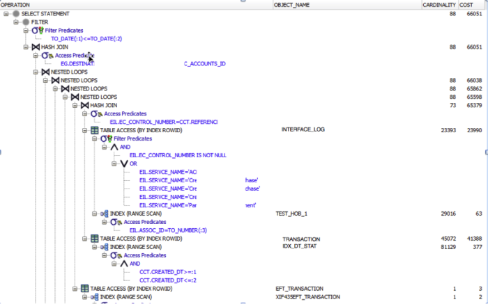
From our review of the explain plan after index creation, we see that the index TEST_HOB_1 was used in an index range scan to limit the record set, and therefore, reduced the cost of the statement by roughly 100,000 to 66,000. This is a theoretical improvement and testing will prove whether or not improved execution times are enough for the end user. Ideally, there would be a measurable reduction in quantifiable server resource utilization verified by looping back for a review of statspack, or just confirming the user experience. If additional resources and system overhead is required, this would have to be addressed before releasing to production. Confirm that any corresponding overhead introduced does not outweigh the improved response times for the system and business.
The benefit of this index is that it is on a single column and lower maintenance than a multi column index. There are cluster waits associated with adding multi-column indexes to a RAC instance that may not be the right solution if multiple sessions across multiple nodes perform frequent DML against the table.
The process is iterative, as we assist the optimizer by providing access paths that did not exist before. Index choices will be guided by decreased costs noted in the explain plan for individual tables and columns in the Where clause. Create a compound index that might satisfy data filters on data, or match the columns joined. Restrict records returned in the Where clause to limit subsets of data in tables with higher cardinality and cost. It is often the combined results of SQL structure changes and index creation together that yield the best results.
Query Diagramming
In his book SQL Tuning, Dan Tow describes the method of query diagramming for analyzing SQL. This method helps the developer and DBA understand the relationship of tables in a SQL statement by providing a visual representation of the work required to fetch results. While representing SQL statements and their joins, the Query Diagramming method is not very SQL like.
A Query Diagram is a directed graph comprised of nodes and links. Nodes represent tables, or table aliases, in the FROM clause. Links represent the joins between tables, where arrows on one end of the link indicate that table contains unique primary key values. Underlined numbers next to the node represent the fraction of rows in each table that will satisfy the filter conditions on that table that are not joins. Non-underlined numbers represent the average number of rows found in the table on that end of the join per matching row on the other end of the join.
Below is a select statement taken from SQL Tuning that we will also use as an example to illustrate these concepts. Figure 4 demonstrates the two nodes required in the query diagram, E and D, short hand for our tables employees and departments.
select
d.department_name,
e.last_name,
e.first_name
from employees e, departments d
where e.department_id=d.department_id
and e.exempt_flag=’Y’
and d.us_based_flag=’Y’;
Figure 4 SQL Query Diagram
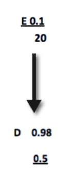
For this query, 10% of the records in employee node satisfy the condition exempt_flag=’Y’ and 50% of the records in department node satisfy the condition US_BASED_FLAG=’Y’. These are the underlined numbers next to E and D in Figure 4. These are filter ratios on the data, and limit the records required to return a result. We may or may not know the size of the table or the column data skews when we perform this exercise. If we have current data, this is worth a lot as we can mine it for answers to our questions with basic selects that follow the filters in the Where clause we are analyzing. If this is a new table that is part of a release, best guess estimates are appropriate.
The non-underlined numbers are join ratios, which is the average number of rows found in the table on that end of the join per matching row from the other table.
The join ratio on the non-unique end of the join is the detail join ratio. In this case, there are many employees per department, due to the one-to-many relationship between the tables. The average count of employees per department is 20.
The join ratio on the unique end of the join is the master join ratio. The master join ratio is between one and zero in one-to-many relationships that are constrained by a foreign key. This foreign key relationship should be confirmed when performing joins between two or more tables. In this case, .98 is the master join ratio because the average employee record matches/joins to a row in the department table 98% of the time.
The value of this query diagram method, and join ratio calculations, is that it helps us visualize the records we are asking a SQL statement to process. The goal is to find the best join order and reduce cost. Often the most optimal access path for a SQL statement is first through indexed access to the first driving table, followed by nested loops through the rest of the joined tables that are also indexed. Our attempts to reduce explain plan cost is ultimately about limiting the number of rows that must be accessed from disk and/or memory. Multi table joins can become very expensive given the many-way joins that occur, and are far are more complex than our example.
We will answer one basic question with this example, which is “what is the appropriate join order for the two tables in this query based on our query diagram cost analysis?” Let’s assume 100 records exist in department and 2,000 in employees.
If starting with the employee table as driving table, per Dan Tow:
- “Using an index on the filter for E, the database must begin by touching 0.1 X C rows in the driving table E.”
- “Following nested loops to master table D, the master join ratio shows that the database will reach 0.1 x C X 0.98 rows of D.”
- “Adding the results of Steps 1 and 2, the total count of table rows touched is (0.1*C)+(0.1*C*0.98).”
- “The total rowcount the database will reach, then, factoring out C and 0.1 from both terms, is C*(0.1*(1+(0.98)), or 0.198*C.”
So, in the case of employee as the driving table, where C is 2,000 (table employee count), the cost is .0198 * 2,000, or 39.6. This estimate of overhead required is a relative value to be compared to other estimates, such as our next one.
If starting with the department table as driving table, per Dan Tow:
- “For every row in D, the database finds on average 20 rows in E, based on the detail join ratio. However, just 98% of the rows in E even match rows in D, so the total rowcount C must be 20/0.98 times larger than the rowcount of D. Conversely, then, the rowcount of D is C*0.98/20.”
- “Following an index to reach only the filter rows on D results in reaching half these rows for the driving table for this alternative, or C * 0.5*.0.98/20.”
- “Following the join to E, then, the database reaches 20 times as many rows in that table: 20 * C * 0.5 * 0.98/20, or C * 0.5 * 0.98.”
- “Adding the two rowcounts and factoring out the common terms as before, find the total cost: C * (0.5 * 0.98 * ((1/20) +1)), or 0.5145*C.”
So, in the case of department as the driving table, where C is 200 (table department count), the cost is .5145 * 200, or 102.9.
Based on this simple query diagramming exercise, we were able to determine that the best plan would use an index on the employee table to filter records and then join to single records in the department table. The cost was 39.6 when the driving table was employee versus a cost of 102.9 when department was the driving table.
This basic exercise is the building block to understanding the performance ramifications associated with SQL statements in conjunction with reading explain plans. Query Diagramming is an abstraction of the work you are asking a SQL statement to execute. The benefit to the developer is the ability to abstract what the SQL statement is asking the database instance to do and review the explain plan to confirm the abstraction. The developer can also use a Query Diagram to represent to an end user what their SQL statement is doing to retrieve results. This can lead to discussions about which records in each table need to be included and evaluated by the SQL based on its Where clause.
By understanding the ramifications of the joins required, and the table sizes and column skews, the developer can tailor the query to include additional filters that limit records accessed in larger tables. Or maybe a full table scan that is now costly due to table growth, can be reviewed to see if an index might assist a filter that was already in place prior. In some cases, a new filter and index might be required. This Query Diagramming exercise might also help a developer and DBA agree that archiving and purging records might be the easiest way to reduce explain plan cost and improve execution times. Limiting datasets analyzed through proper data life cycle management saves on storage consumption, Disk I/O utilization and CPU utilization.
Note: The Oracle Optimizer is certainly sophisticated enough to figure out the driving table depending on the access paths available to it, given our simple example above. The problem is the Optimizer cannot choose access paths that are not available to it, and Query Diagramming can reveal what indexes to consider based on the tables being accessed by your SQL. By learning how the Optimizer responds to your trial and error tuning attempts, you will improve your ability to generate efficient explain plans
Dan Tow’s book SQL Tuning is recommended for developers and DBAs alike who want more background on how to approach SQL tuning problems.
Conclusion
This Oracle performance tuning series was meant to provide a general framework for diagnosing performance problems with the most basic tools available. Understanding the concepts in this blog series will help when leveraging many of the excellent performance monitoring and tuning tools available to DBAs and developers today. This series should give you some rudimentary concept as to why a performance tool may be making certain recommendations about poorly performing SQL in your instance.
For those organizations that have purchased Oracle’s Diagnostics and Tuning Pack and have access to features such as the SQL Tuning Advisor and SQL Access Advisor, very quick analysis can be made of expensive and long running statements. These Oracle tools can provide suggestions for SQL profiles or indexes that can significantly reduce explain plan expense and associated resource utilization. However, not all instances require these additional Oracle tuning features, especially if the environment contains efficient code and is fairly static. In dynamic environments with inefficient SQL, frequent DDL releases, and poor data life cycle management, these additional tuning tools and methods start to become mandatory.
References:
Tow, Dan SQL Tuning O’Reilly Media Inc., 2004
Shee, Richmond and Kirtikumar Deshpande, K. Gopalakrishnan Oracle Wait Interface: A Practical Guide to Performance Diagnostics and Tuning (Oracle Press Series) (More System/Session Related) 2004
Millsap, Cary and Jeff Holt Optimizing Oracle Performance Boston: O’Reilly Media Inc., 2003